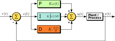
What is PID?
This is a quick post on what PID is and how to implement it.
For startes, PID stands for Proportional-Integral-Derivative. And PID is a closed-loop feedback controller. That means that when the controller outputs a value, that output will change the input, which will result in another different output to be produced. And this systems goes on and on until the main program is terminated.
When are PID Controllers used?
Well, in almost any application that needs to be actively controlled. Such as: autopilot UAVs, self-balancing robots, drones, battery chargers, etc.
So what exactly are PID controllers?
Well, let’s start off with the proportional part:
As you might of thought, this part produces a value proportional to the error. For example: let’s assume we are making a drone. And the orientation sensor detects that we are tilting by 20 degrees. And let’s say that the P Value (or the Proportional Value) is 0.5. Then the output of the P part will be -20*0.5 which is -10 degrees. We say negative, because our target value, which is 0 minus our error is a negative value. If our error was 90 degrees, then the P Value would be -45 degrees. Essentially, the output is proportional to the error with respect to the P Value. However, this alone isn’t very affective in the real world. Because in the real world there is momentum. Which means our system will overshoot, which causes oscillations in the system.
Next, what does the Integral Part mean. And to better understand why this is important, let’s first know why the Derivative term is there.
the D term, or the Derivative:
If you have noticed, the I and D parts are names commonly used in Calculus. This is because we actually are using concepts from Calculus. The Derivative term looks at our error ‘curve’ over time. Actually, it’s not over time but this is what I mean: Imagine our error values are being plotted on an x-y plane, where the x-axis is time and the y-axis is the error. Now this will form some sort of ‘curve’ (I just mean a plot or graph). And by definition, the Derivative term is looking at the slope of our curve. Or basically, how fast are we going away or to our target value (in most systems this will be 0 or the x-axis)? And the D term changes accordingly to that value. Let’s go through an example (sticking to the one above): Now let’s assume our D Value is say 10. And the slope of the error curve is negative, say -2. Then the output of the D function is (D Value * slope) or (10) * (-2) = -20. So we will be adding a negative value of 20 to the output of the P function which is -30. This will cause a bit more aggressive of a response, since our slope is somewhat high; which means we are moving fast, so we require a more aggressive counter. This term, where we slightly modify the output of the P term, depending on how fast we’re moving results in NO OVERSHOOTING! This alone is a pretty good system. However, there are some scenarios where the error is not at the target but the specific P and D terms aren’t affective at getting it back to the target. This is when the Intergal term comes in.
Finally, the Integral term:
This looks at the area under our curve relative to our target value, the line y=targetVal. How it calculates the area isn’t exact, but it is an apporximation. The equation for the Integral term is adding our old area term to the multiplication of our error value and the change in time (or the time interval which we last calculated our error).
In Arduino Code:
pitchErrorArea=pitchErrorArea+(pitchError*dt);
And if you’ve noticed, this is actually the area of a rectangle, where the length is the time intevral and the height is the error. And you’ve probably also noticed that this doesn’t always match up with the actual graph, but it’s a pretty good approximation.
Now, this is when the Integral term is useful:
Let’s go back to the graph. Our system without the Integral term is pretty good, but it isn’t affective at long term stuff. Like when our error is really close to the target, but isn’t actually equal to it, and over time, this makes a difference. So as a solution, we take the area of the part between our target and the graph, and add them up over time (this is called Integrating) to get our current area. And we divide this area by a sufficiently large number (or multiply this area by a sufficiently small number, like 0.0001, which is our Integral part) which we then add to our correcting value; which will over time be making small adjustments to get us closer to our target. And that completes our PID system.
If you want a visual:

Also, depending on the system, you will need to play around with the P, I, and D values to perfectly tune it to your specific system. This takes lots of trial and error, but is definetly worth it!
If you want more resources:
Hope you learned something!!
Subscribe to Burak Ayyorgun
Get the latest posts delivered right to your inbox